論文読み 2017, Dynamic Routing Between Capsules

元ネタ: Dynamic Routing Between Capsules, Sabour et al. NIPS, 2017 (第一著者のSara氏にもっと敬意を)

人間の視覚は極僅かな凝視点(fixation points)を選んで，その近くだけを高解像度に処理している． 例えば顔を認識する時，有る凝視点は口，またある凝視点は鼻・・・といった風に凝視点を選んでいるとしよう． この論文では，ある凝視点(口を見ている凝視点とする)を処理する時，単に口の情報だけでなくもっと多くの情報を得ていると仮定し，さらに我々の視覚はそれぞれの凝視点から得た情報を構文木のように構造化していると仮定する． ヒトの視覚はmulti-layer neural networkであることがわかっていて，さらにそれぞれのlayerは多くの”capsule”と呼ばれるneuron群に分割でき(これは多分筆者の想像)，見られているものに関係したcapsuleだけが発火して構文木を構成している. 低次の(目玉に近い)layerでのcapsuleの発火に従ってより高次のlayerでのcapsuleの発火が決定されていくという処理の繰り返しが起きているのである． capsuleの中のそれぞれのneuronは見ている対象の様々な属性(位置，大きさ，方向，deformation,測度,反射,etc.)を表現している．
この論文では以上の仮定の計算モデルを実装し，それが画像処理でうまく働いたことを示した．

論文読み 2015, 2016, DeepLab v1/v2

元ネタ:
Liang-Chieh Chen and George Papandreou and Iasonas Kokkinos and Kevin Murphy and Alan L Yuille, Semantic Image Segmentation with Deep Convolutional Nets and Fully Connected CRFs, ICLR, 2015.

Liang-Chieh Chen, George Papandreou, Iasonas Kokkinos, Kevin Murphy, Alan L. Yuille, DeepLab: Semantic Image Segmentation with Deep Convolutional Nets, Atrous Convolution, and Fully Connected CRFs, arXiv preprint, 2016

“DeepLab”の初出とその直後に出た論文． 最新のDeepLabv3は現在のstate-of-the-artである．

DeepLabの特徴を3つ挙げる.
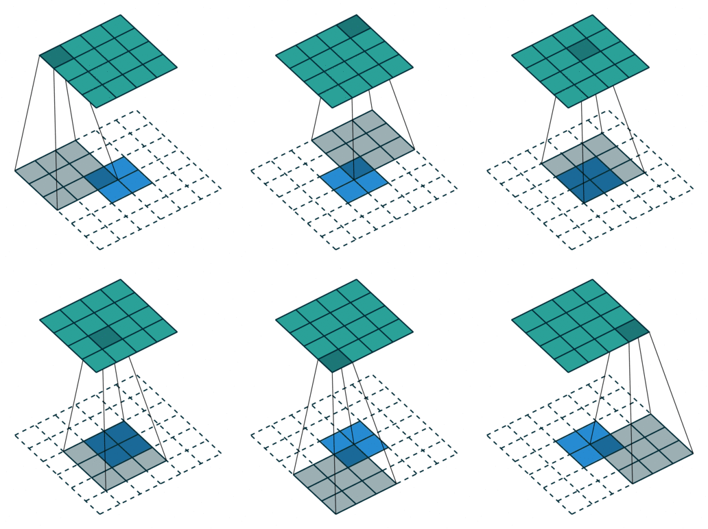
1. poolingによるdownsamplingのかわりにAtrous Convolution(fig.1)を使って，downsamplingのときに得られる一つ一つの特徴量がより広い範囲の入力元を反映することになる.Atrous ConvolutionはDilated Convolutionとも呼ばれる． PyTorchではtorch.nn.Conv2dのdilation引数で設定できる.
figure 1. from vdumoulin/conv_arithmetic
2. 画面いっぱいに写っていようと画面の片隅に写っていようと猫は猫であるように，image segmentationではscale invarianceを考慮しなければならない． 著者はAtrous Convolutionのdilationを様々に設定することでこれに対処している(fig.2). 著者はこの技法を”atrous spatial pyramid pooling”(ASPP)と呼んでいる.

figure 2, from Liang-Chieh et al. 2016
3. bilinaer upsamplingによってfeature mapを引き伸ばすのだが，その直後にfully-connected Conditional Random Field (CRF)を用いる． CRFはdeep-learning以前のimage segmentationでよく用いられてきた技法である.画像の隣り合った画素のペアを考えて，その2つが同じobjectに入るか否かを計算していくのがUnary(Basic) CRFである(fig.3a). Fully Connecetd CRFでは文字通りある画素とその他の任意の画素のペアが同じobjectに入るか否かを考慮する(fig.3b)． 当然Fully Connected CRFはそのままだと極めて計算量が大きいが，Krahenbuhl and Koltun, 2011．は平均場近似を導入して高速化を行い，exhaustiveな計算に近い結果を得た(fig.4).

figure 3. from https://www.cs.auckland.ac.nz/courses/compsci708s1c/lectures/glect-html/topic4c708fsc.htm

figure 4, from Krahenbuhl and Koltun, 2011

モデル概観, from Liang-Chieh et al. 2015

似たアーキテクチャで注目されているのにZheng et al. Conditional Random Fields as Recurrent Neural Networksがある．

(詳しい議論はDeepLabv3の論文読みで)

論文読み 2015, SegNet: A Deep Convolutional Encoder-Decoder Architecture for Image Segmentation

元ネタ: Vijay Badrinarayanan, Alex Kendall, Roberto Cipolla,
“SegNet: A Deep Convolutional Encoder-Decoder Architecture for Image Segmentation.” PAMI, 2017.
(arxivで2015なのにPAMIで2017ってどういうことなの・・・)

自動運転のAIのために開発されたimage segmentation技術．
構造はU-Netによく似ている(fig.1)が，feature mapの引き伸ばしをmax-unpooling( PyTorch)によって行うことでモデルを単純化し，リアルタイムな処理に向いたアルゴリズムになっている
figure 1, SegNetウェブサイトより

論文読み 2015, U-Net: Convolutional Networks for Biomedical Image Segmentation

元ネタ: Ronneberger, Olaf; Fischer, Philipp; Brox, Thomas,
U-Net: Convolutional Networks for Biomedical Image Segmentation. Medical Image Computing and Computer-Assisted Intervention (MICCAI), Springer, LNCS, Vol.9351: 234–241, 2015

細胞や臓器といった生物学の画像に特化したimage segmentationの技法．
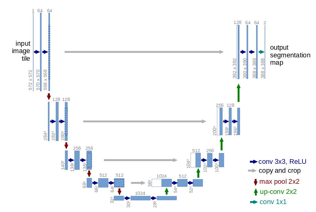
FCNがfeature mapの縦横を急激に縮めたり引き伸ばすのに対して，U-Netでは縮めるのは1/2倍づつ，引き伸ばすのも2倍づつとしている． またfeature mapの縦横をa倍するたびにfeature mapの数を1/a倍している. fig.1から見て取れるように，U-Netを図示するとほとんど左右対称になっていて，左側の，特徴を抽出しつつ画像を圧縮していく部分をencoder,特徴量に対応したsegmentationを保持しながら画像を引き伸ばしていく部分をdecoderという． Encoderで得られた特徴量は縦横比が一致するように切り抜かれてから対応するfeature volumeと結合し，さらにupsamplingされていく． 引き伸ばしには”up-convolution”(おそらくFCNと同じヤツ)を使う．

生物学的画像の特徴として，かなりグニャグニャ歪めてもその実体(細胞・臓器)はクラスとして不変だから，そのようなdata augmentationを工夫している．

わかりやすい実装, ZijunDeng

DataLoaderの使い方

DataLoaderにはDataset型を食わせればいい
例:Kaixhin/FCN-semantic-segmentation/data.py

import os
import random
from PIL import Image
import torch
from torch.utils.data import Dataset


# Labels: -1 license plate, 0 unlabeled, 1 ego vehicle, 2 rectification border, 3 out of roi, 4 static, 5 dynamic, 6 ground, 7 road, 8 sidewalk, 9 parking, 10 rail track, 11 building, 12 wall, 13 fence, 14 guard rail, 15 bridge, 16 tunnel, 17 pole, 18 polegroup, 19 traffic light, 20 traffic sign, 21 vegetation, 22 terrain, 23 sky, 24 person, 25 rider, 26 car, 27 truck, 28 bus, 29 caravan, 30 trailer, 31 train, 32 motorcycle, 33 bicycle
num_classes = 20
full_to_train = {-1: 19, 0: 19, 1: 19, 2: 19, 3: 19, 4: 19, 5: 19, 6: 19, 7: 0, 8: 1, 9: 19, 10: 19, 11: 2, 12: 3, 13: 4, 14: 19, 15: 19, 16: 19, 17: 5, 18: 19, 19: 6, 20: 7, 21: 8, 22: 9, 23: 10, 24: 11, 25: 12, 26: 13, 27: 14, 28: 15, 29: 19, 30: 19, 31: 16, 32: 17, 33: 18}
train_to_full = {0: 7, 1: 8, 2: 11, 3: 12, 4: 13, 5: 17, 6: 19, 7: 20, 8: 21, 9: 22, 10: 23, 11: 24, 12: 25, 13: 26, 14: 27, 15: 28, 16: 31, 17: 32, 18: 33, 19: 0}
full_to_colour = {0: (0, 0, 0), 7: (128, 64, 128), 8: (244, 35, 232), 11: (70, 70, 70), 12: (102, 102, 156), 13: (190, 153, 153), 17: (153, 153, 153), 19: (250, 170, 30), 20: (220, 220, 0), 21: (107, 142, 35), 22: (152, 251, 152), 23: (70, 130, 180), 24: (220, 20, 60), 25: (255, 0, 0), 26: (0, 0, 142), 27: (0, 0, 70), 28: (0, 60,100), 31: (0, 80, 100), 32: (0, 0, 230), 33: (119, 11, 32)}


class CityscapesDataset(Dataset):
  def __init__(self, split='train', crop=None, flip=False):
    super().__init__()
    self.crop = crop
    self.flip = flip
    self.inputs = []
    self.targets = []

    for root, _, filenames in os.walk(os.path.join('leftImg8bit_trainvaltest', 'leftImg8bit', split)):
      for filename in filenames:
        if os.path.splitext(filename)[1] == '.png':
          filename_base = '_'.join(filename.split('_')[:-1])
          target_root = os.path.join('gtFine_trainvaltest', 'gtFine', split, os.path.basename(root))
          self.inputs.append(os.path.join(root, filename_base + '_leftImg8bit.png'))
          self.targets.append(os.path.join(target_root, filename_base + '_gtFine_labelIds.png'))

  def __len__(self):
    return len(self.inputs)

  def __getitem__(self, i):
    # Load images and perform augmentations with PIL
    input, target = Image.open(self.inputs[i]), Image.open(self.targets[i])
    # Random uniform crop
    if self.crop is not None:
      w, h = input.size
      x1, y1 = random.randint(0, w - self.crop), random.randint(0, h - self.crop)
      input, target = input.crop((x1, y1, x1 + self.crop, y1 + self.crop)), target.crop((x1, y1, x1 + self.crop, y1 + self.crop))
    # Random horizontal flip
    if self.flip:
      if random.random() < 0.5:
        input, target = input.transpose(Image.FLIP_LEFT_RIGHT), target.transpose(Image.FLIP_LEFT_RIGHT)

    # Convert to tensors
    w, h = input.size
    input = torch.ByteTensor(torch.ByteStorage.from_buffer(input.tobytes())).view(h, w, 3).permute(2, 0, 1).float().div(255)
    target = torch.ByteTensor(torch.ByteStorage.from_buffer(target.tobytes())).view(h, w).long()
    # Normalise input
    input[0].add_(-0.485).div_(0.229)
    input[1].add_(-0.456).div_(0.224)
    input[2].add_(-0.406).div_(0.225)
    # Convert to training labels
    remapped_target = target.clone()
    for k, v in full_to_train.items():
      remapped_target[target == k] = v
    # Create one-hot encoding
    target = torch.zeros(num_classes, h, w)
    for c in range(num_classes):
      target[c][remapped_target == c] = 1
return input, target, remapped_target # Return x, y (one-hot), y (index)

論文読み 2015, Fully Convolutional Networks for Semantic Segmentation

元ネタ: Long, J., Shelhamer, E., & Darrell, T. Fully convolutional networks for semantic segmentation. In CVPR, 2015.

Introduction

CNNではレイヤーを重ねるに連れて特徴量(この論文内ではsemanticsと呼んでいる)が抽出されていくが，一方でそれが元の画像のどこに有るのか(location)という情報は失われてしまう． これはimage segmentationの場合に不利に働き，普通に出力層を元の画像と対応したピクセルの並びと考えて学習しても，極めて荒い情報しか得られない. そこで著者はFully Convolutional Net (FCN, 全ての層がconvolutionであるnet)を利用した． FCNは空間的情報を前の方のlayerから”skip architecture”によって持ってきて，semanticsと統合してpixelごとの属性を推測する．
LeNetやVGGのようなclassification用のネットワークからのtransfer learningによって学習を高速化しているのもこの論文の特徴である．

Fully convolutional networks

$\mathbf{x}_{ij}$を(layerの)入力の$(i, j)$のところに有るデータとし，$\mathbf{y}_{ij}$を(layerの)出力のそれとすると，convolutionやそれにともなうpoolingやactivationのlayer (stageと呼んだほうが通りがいいか)というのは,
$$\mathbf{y}_{ij} = f_{ks} (\{\mathbf{x}_{si+\delta i, sj+\delta_j}\} | 0\leq \delta_i, \delta_j \leq k)$$
と書ける.ただし$k$はfilterの幅,$s$はストライドの幅とする.
複数のlayerの合成の表現は
$$f_{ks} \circ g_{k's'} = (f \circ g)_{k'+(k-1)s', ss'}$$
と書ける．したがって,全結合層を持たないCNNは(これをFully Convolutional Netowork, FCNという)この合成の形で書けることになる． また，FCNは任意の大きさの画像を入力と出来る．

Adapting classifiers for dense prediction

ふつうのCNNの最後の方には全結合層が有るが，これを，その直前のlayerからの入力(h x w x d)を，h x w x dのfilterでconvolutionしたものだと考えることが出来る(fig.1)．
しかしこれでは出力層では空間的情報が著しく失われているので，出力層をdense(密)にするというのが著者の重要な仕事といえる．

Upsampling is backwards strided convolution

(vdumoulin/conv_arithmetic, MIT license)

Segmentation Architectue

Combining what and where

空間的情報を前の方のlayerから”skip architecture”によって持ってきて，semanticsと統合してpixelごとの属性を推測する
skip architectureがどうなっているのかわからないので今度pytorch実装を見る
（ただの足し算だった）

論文読み 2015, Rethinking the Inception Architecture for Computer Vision

元ネタ: Szegedy, Christian & Vanhoucke, Vincent & Ioffe, Sergey & Shlens, Jon & Wojna, ZB. (2015). Rethinking the Inception Architecture for Computer Vision. . 10.1109/CVPR.2016.308.

Introduction

Inception1を改良して，Inception-v2並びにv3を開発した．

Inception-v3はInception-v2のAuxiliary classifierにbatch-normalizationを追加したモデルと言える.

General Design Principles

Inception2の改良を試みた際に得たいくつかの経験則を挙げている.
1. layerを急に狭める(representational bottleneck)ことを避ける. ネットワークを通して結局は同じ次元に落とし込むにしても，あるlayerの次のlayerに移る時に急に次元がさげてはならない.
2. 高次元のlayerは局所的に処理しやすい. convoluationにおいてtileごとのactivationを増加させると,抽出される特徴がよりdisentangledになる.
3. 低次元な埋め込みによって，空間的なaggregationをほとんどあるいは全くロスなくおこなえる．例えば(3x3)のconvolutionを行う前に1x1のconvolutionでそのlayerへの入力を低次元に埋め込み,より効率的に3x3のconvolutionを行えて，かつ情報のロスはわずかである．
4. ネットワークの幅と深さのバランスをとる． 片方を増加させることでNNの性能を向上させることは可能だが，療法を同時に増加させることで計算量の増大を抑えつつ性能を向上させられる．

Factorizing Convolutions with Larger Filter Size

Inception3では1x1のconvolutionで次元削減した上で5x5や3x3のconvolutionを行ったが，他のfactorizing convolutionを試している.

3.1 Factorization into smaller convolutions

5x5 や 7x7のconvolutionは非常に計算のコストが大きいので，より小さいconvolutionを複数重ねることで似たようなconvolutionを実現する.(fig.1)

3.2 Spatial Factorization into Asymmetric Convolutions

nxnのconvolutionを1xnとnx1のconvolutionの2段構えで処理する(fig.2)と計算効率は飛躍的に向上する．実験では，lower layers(inputに近いlayer)でこれを行うとうまく行かないが，12x12や20x20のconvolutionでは非常に効果的であった.

4. Utility of Auxiliary Classifiers

Inception4で複数のclassifierを導入して勾配消失を防ごうとしたが，Lee et al[^2]と対照的に著者は複数のclassifierによる収束の高速化は確認できなかった一方で，classifierが一つであるよりも僅かに分類性能の向上を認めた．著者らは複数のclassifierがregularizerとして働いているのではないかと考えている．

5. Efficient Grid Size Reduction

fig.2の方法でfeature mapを効率的に増やしているらしい

figure 2

7. Model Regularization via Label Smoothing (LSR)

training setにおけるラベル$k \in \{1,...,K\}$の分布$u(k)$を,example $x$とは関係なく得る(traing setにおける$k$の出現確率かと思ったがそうでもないらしい)，またsmoothing parameter $\epsilon$を定義する． ground truth $y$のexample $x$に対して，ground truthの分布$q(k|x)=\delta_{k,y}$:(ディラックのデルタ)を，
$q'(k|x)=(1-\epsilon) \delta_{k,y} + \epsilon u(k)$によって書き換える．
例えば$u(k)=1/K$とすれば
$$q'(k)=(1-\epsilon)\delta_{k,y} + \frac{\epsilon}{K}$$
である．

---

1. Christian Szegedy, Wei Liu, Yangqing Jia, Pierre Sermanet, Scott Reed, Dragomir Anguelov, Dumitru Erhan, Vincent Vanhoucke, Andrew Rabinovich, Going Deeper with Convolutions, In CVPR, 2014 ↩
2. Christian Szegedy, Wei Liu, Yangqing Jia, Pierre Sermanet, Scott Reed, Dragomir Anguelov, Dumitru Erhan, Vincent Vanhoucke, Andrew Rabinovich, Going Deeper with Convolutions, In CVPR, 2014 ↩
3. Christian Szegedy, Wei Liu, Yangqing Jia, Pierre Sermanet, Scott Reed, Dragomir Anguelov, Dumitru Erhan, Vincent Vanhoucke, Andrew Rabinovich, Going Deeper with Convolutions, In CVPR, 2014 ↩
4. Christian Szegedy, Wei Liu, Yangqing Jia, Pierre Sermanet, Scott Reed, Dragomir Anguelov, Dumitru Erhan, Vincent Vanhoucke, Andrew Rabinovich, Going Deeper with Convolutions, In CVPR, 2014 ↩