2017年11月23日木曜日

論文読み 2015, Fully Convolutional Networks for Semantic Segmentation

元ネタ: Long, J., Shelhamer, E., & Darrell, T. Fully convolutional networks for semantic segmentation. In CVPR, 2015.

Introduction

CNNではレイヤーを重ねるに連れて特徴量(この論文内ではsemanticsと呼んでいる)が抽出されていくが,一方でそれが元の画像のどこに有るのか(location)という情報は失われてしまう. これはimage segmentationの場合に不利に働き,普通に出力層を元の画像と対応したピクセルの並びと考えて学習しても,極めて荒い情報しか得られない. そこで著者はFully Convolutional Net (FCN, 全ての層がconvolutionであるnet)を利用した. FCNは空間的情報を前の方のlayerから”skip architecture”によって持ってきて,semanticsと統合してpixelごとの属性を推測する.
LeNetやVGGのようなclassification用のネットワークからのtransfer learningによって学習を高速化しているのもこの論文の特徴である.

Fully convolutional networks

を(layerの)入力ののところに有るデータとし,を(layerの)出力のそれとすると,convolutionやそれにともなうpoolingやactivationのlayer (stageと呼んだほうが通りがいいか)というのは,

と書ける.ただしはfilterの幅,はストライドの幅とする.
複数のlayerの合成の表現は

と書ける.したがって,全結合層を持たないCNNは(これをFully Convolutional Netowork, FCNという)この合成の形で書けることになる. また,FCNは任意の大きさの画像を入力と出来る.

Adapting classifiers for dense prediction

ふつうのCNNの最後の方には全結合層が有るが,これを,その直前のlayerからの入力(h x w x d)を,h x w x dのfilterでconvolutionしたものだと考えることが出来る(fig.1).
しかしこれでは出力層では空間的情報が著しく失われているので,出力層をdense(密)にするというのが著者の重要な仕事といえる.

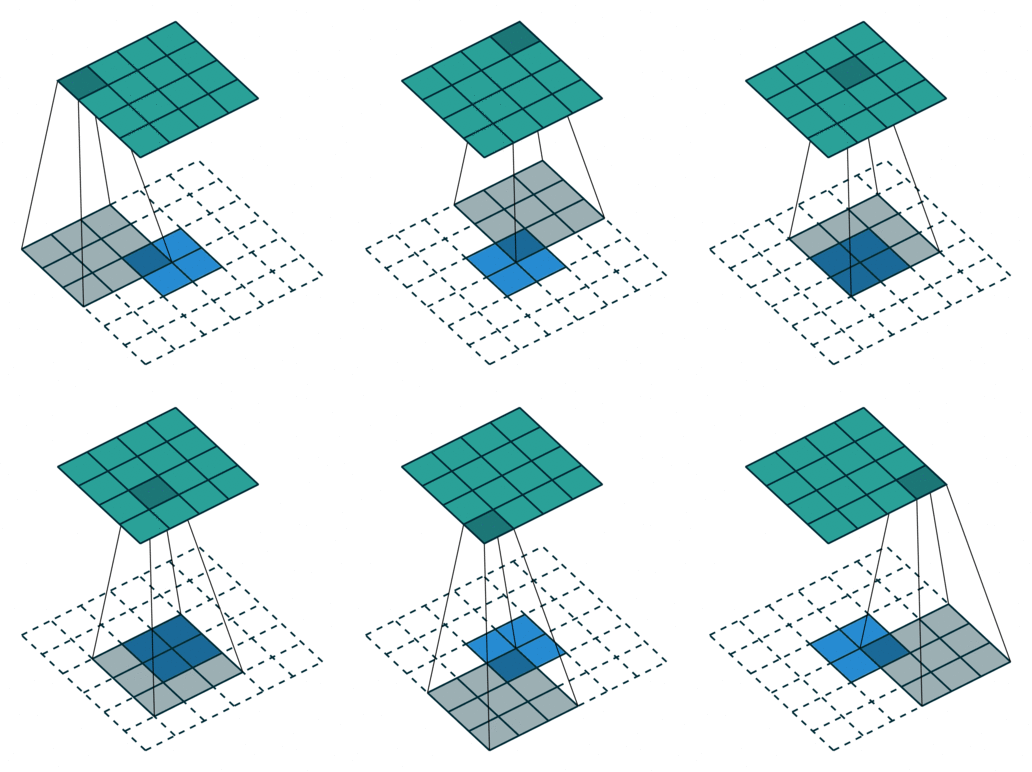
Upsampling is backwards strided convolution

enter image description here
(vdumoulin/conv_arithmetic, MIT license)

Segmentation Architectue

Combining what and where

enter image description here
空間的情報を前の方のlayerから”skip architecture”によって持ってきて,semanticsと統合してpixelごとの属性を推測する
skip architectureがどうなっているのかわからないので今度pytorch実装を見る
(ただの足し算だった)

2017年11月22日水曜日

論文読み 2015, Rethinking the Inception Architecture for Computer Vision

元ネタ: Szegedy, Christian & Vanhoucke, Vincent & Ioffe, Sergey & Shlens, Jon & Wojna, ZB. (2015). Rethinking the Inception Architecture for Computer Vision. . 10.1109/CVPR.2016.308.

Introduction

Inception1を改良して,Inception-v2並びにv3を開発した.

Inception-v3はInception-v2のAuxiliary classifierにbatch-normalizationを追加したモデルと言える.

General Design Principles

Inception2の改良を試みた際に得たいくつかの経験則を挙げている.
1. layerを急に狭める(representational bottleneck)ことを避ける. ネットワークを通して結局は同じ次元に落とし込むにしても,あるlayerの次のlayerに移る時に急に次元がさげてはならない.
2. 高次元のlayerは局所的に処理しやすい. convoluationにおいてtileごとのactivationを増加させると,抽出される特徴がよりdisentangledになる.
3. 低次元な埋め込みによって,空間的なaggregationをほとんどあるいは全くロスなくおこなえる.例えば(3x3)のconvolutionを行う前に1x1のconvolutionでそのlayerへの入力を低次元に埋め込み,より効率的に3x3のconvolutionを行えて,かつ情報のロスはわずかである.
4. ネットワークの幅と深さのバランスをとる. 片方を増加させることでNNの性能を向上させることは可能だが,療法を同時に増加させることで計算量の増大を抑えつつ性能を向上させられる.

Factorizing Convolutions with Larger Filter Size

Inception3では1x1のconvolutionで次元削減した上で5x5や3x3のconvolutionを行ったが,他のfactorizing convolutionを試している.

3.1 Factorization into smaller convolutions

5x5 や 7x7のconvolutionは非常に計算のコストが大きいので,より小さいconvolutionを複数重ねることで似たようなconvolutionを実現する.(fig.1)
enter image description here

3.2 Spatial Factorization into Asymmetric Convolutions

nxnのconvolutionを1xnとnx1のconvolutionの2段構えで処理する(fig.2)と計算効率は飛躍的に向上する.実験では,lower layers(inputに近いlayer)でこれを行うとうまく行かないが,12x12や20x20のconvolutionでは非常に効果的であった.

4. Utility of Auxiliary Classifiers

Inception4で複数のclassifierを導入して勾配消失を防ごうとしたが,Lee et al[^2]と対照的に著者は複数のclassifierによる収束の高速化は確認できなかった一方で,classifierが一つであるよりも僅かに分類性能の向上を認めた.著者らは複数のclassifierがregularizerとして働いているのではないかと考えている.

5. Efficient Grid Size Reduction

fig.2の方法でfeature mapを効率的に増やしているらしい
enter image description here
figure 2

7. Model Regularization via Label Smoothing (LSR)

training setにおけるラベルの分布を,example とは関係なく得る(traing setにおけるの出現確率かと思ったがそうでもないらしい),またsmoothing parameter を定義する. ground truth のexample に対して,ground truthの分布:(ディラックのデルタ)を,
によって書き換える.
例えばとすれば

である.


  1. Christian Szegedy, Wei Liu, Yangqing Jia, Pierre Sermanet, Scott Reed, Dragomir Anguelov, Dumitru Erhan, Vincent Vanhoucke, Andrew Rabinovich, Going Deeper with Convolutions, In CVPR, 2014 ↩
  2. Christian Szegedy, Wei Liu, Yangqing Jia, Pierre Sermanet, Scott Reed, Dragomir Anguelov, Dumitru Erhan, Vincent Vanhoucke, Andrew Rabinovich, Going Deeper with Convolutions, In CVPR, 2014 ↩
  3. Christian Szegedy, Wei Liu, Yangqing Jia, Pierre Sermanet, Scott Reed, Dragomir Anguelov, Dumitru Erhan, Vincent Vanhoucke, Andrew Rabinovich, Going Deeper with Convolutions, In CVPR, 2014 ↩
  4. Christian Szegedy, Wei Liu, Yangqing Jia, Pierre Sermanet, Scott Reed, Dragomir Anguelov, Dumitru Erhan, Vincent Vanhoucke, Andrew Rabinovich, Going Deeper with Convolutions, In CVPR, 2014 ↩

2017年11月21日火曜日

論文読み 2014, Going Deeper with Convolutions

Introduction

Szegedy et al. (2014)1ではより深いDNNを実現するためにInception moduleを導入し,22層からなるGoogLenetを開発し,ほぼ同じ計算量で性能の向上を実現している.VGGNet2は精度の点ではGoogLeNetと同程度だが,従来のCNNを深くしただけで,非常に計算量が大きいという欠点が有る.
ただ単にDNNを大きくすることは計算量を増大させると同時に必要なtraining dataを莫大にしてしまう. これを克服するためにsparsityを用いるのだが,sparse行列の演算は現在の計算機では扱いづらい. 従来は”spatial domain”においてconvolutionを導入してsparsityを実現してきたが,著者は”filter-level”でsparsityを実現し,しかも複数のsparse行列の演算を1つのdense行列の演算として近似して効率よく計算する方法を開発した.
Inception moduleとは通常のconvolutionの代わりに挿入される,複数のconvolutionをひとまとめにしたレイヤーと言える.
CNNでは局所的な統計量のクラスターが前のレイヤーから後ろのレイヤーに渡されていくわけだが,その受け渡されたレイヤーでももとの局所性は保存されているから,ついにはその局所的な統計量たちの殆どがfeature mapのうちの1x1の部分のそれぞれに格納されることになる. Inception moduleでは1x1のフィルタに加え,1x1の部分に収まりきらない局所統計量をとらえるため,3x3と5x5のフィルタも加え,ついでにpoolingも加えている(fig.1.a), .
大量のfeature mapが有る上に5X5のconvolutionを行うのは非常に計算が重いので,1x1のconvolutionを適当な枚数のfeature mapを作るように掛けて次元圧縮してからそれに3x3や5x5のconvolutionを施す(fig.1.b), (table1, n5x5redやn3x3redが次元圧縮した後の次元数).
計算上の理由から,Inception moduleはDNNのhigher layerにおいてのみ挿入される. GoogLeNetは合計で22のlayerからなるが,当時としてはあまりに深いネットワークなので,中頃の層にもclassifierを追加して(fig.2)勾配消失を軽減するとともに,regularizationを実現していると著者は考えている.

enter image description here
figure1

Table1, PyTorch実装,kuangliu, MIT license

import torch
import torch.nn as nn
import torch.nn.functional as F

from torch.autograd import Variable


class Inception(nn.Module):
    def __init__(self, in_planes, n1x1, n3x3red, n3x3, n5x5red, n5x5, pool_planes):
        super(Inception, self).__init__()
        # 1x1 conv branch
        self.b1 = nn.Sequential(
            nn.Conv2d(in_planes, n1x1, kernel_size=1),
            nn.BatchNorm2d(n1x1),
            nn.ReLU(True),
        )

        # 1x1 conv -> 3x3 conv branch
        self.b2 = nn.Sequential(
            nn.Conv2d(in_planes, n3x3red, kernel_size=1),
            nn.BatchNorm2d(n3x3red),
            nn.ReLU(True),
            nn.Conv2d(n3x3red, n3x3, kernel_size=3, padding=1),
            nn.BatchNorm2d(n3x3),
            nn.ReLU(True),
        )

        # 1x1 conv -> 5x5 conv branch
        self.b3 = nn.Sequential(
            nn.Conv2d(in_planes, n5x5red, kernel_size=1),
            nn.BatchNorm2d(n5x5red),
            nn.ReLU(True),
            nn.Conv2d(n5x5red, n5x5, kernel_size=3, padding=1),
            nn.BatchNorm2d(n5x5),
            nn.ReLU(True),
            nn.Conv2d(n5x5, n5x5, kernel_size=3, padding=1),
            nn.BatchNorm2d(n5x5),
            nn.ReLU(True),
        )

        # 3x3 pool -> 1x1 conv branch
        self.b4 = nn.Sequential(
            nn.MaxPool2d(3, stride=1, padding=1),
            nn.Conv2d(in_planes, pool_planes, kernel_size=1),
            nn.BatchNorm2d(pool_planes),
            nn.ReLU(True),
        )

    def forward(self, x):
        y1 = self.b1(x)
        y2 = self.b2(x)
        y3 = self.b3(x)
        y4 = self.b4(x)
        return torch.cat([y1,y2,y3,y4], 1)


class GoogLeNet(nn.Module):
    def __init__(self):
        super(GoogLeNet, self).__init__()
        self.pre_layers = nn.Sequential(
            nn.Conv2d(3, 192, kernel_size=3, padding=1),
            nn.BatchNorm2d(192),
            nn.ReLU(True),
        )

        self.a3 = Inception(192,  64,  96, 128, 16, 32, 32)
        self.b3 = Inception(256, 128, 128, 192, 32, 96, 64)

        self.maxpool = nn.MaxPool2d(3, stride=2, padding=1)

        self.a4 = Inception(480, 192,  96, 208, 16,  48,  64)
        self.b4 = Inception(512, 160, 112, 224, 24,  64,  64)
        self.c4 = Inception(512, 128, 128, 256, 24,  64,  64)
        self.d4 = Inception(512, 112, 144, 288, 32,  64,  64)
        self.e4 = Inception(528, 256, 160, 320, 32, 128, 128)

        self.a5 = Inception(832, 256, 160, 320, 32, 128, 128)
        self.b5 = Inception(832, 384, 192, 384, 48, 128, 128)

        self.avgpool = nn.AvgPool2d(8, stride=1)
        self.linear = nn.Linear(1024, 10)

    def forward(self, x):
        out = self.pre_layers(x)
        out = self.a3(out)
        out = self.b3(out)
        out = self.maxpool(out)
        out = self.a4(out)
        out = self.b4(out)
        out = self.c4(out)
        out = self.d4(out)
        out = self.e4(out)
        out = self.maxpool(out)
        out = self.a5(out)
        out = self.b5(out)
        out = self.avgpool(out)
        out = out.view(out.size(0), -1)
        out = self.linear(out)
        return out

# net = GoogLeNet()
# x = torch.randn(1,3,32,32)
# y = net(Variable(x))
# print(y.size())

enter image description here
figure 2

figureは原論文より


  1. Christian Szegedy, Wei Liu, Yangqing Jia, Pierre Sermanet, Scott Reed, Dragomir Anguelov, Dumitru Erhan, Vincent Vanhoucke, Andrew Rabinovich, Going Deeper with Convolutions, In CVPR, 2014 ↩
  2. K. Simonyan and A. Zisserman. Very deep convolutionalnetworks for large-scale image recognition.arXiv preprint arXiv:1409.1556, 2014. ↩